How to Build a KPI Dashboard in Excel
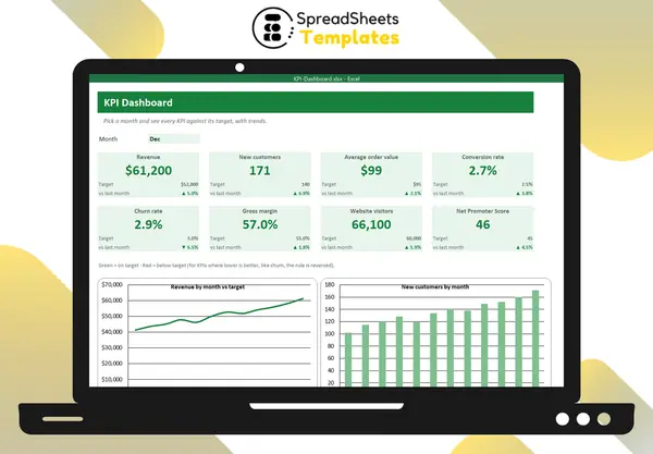
A KPI dashboard puts the few numbers that matter most on one screen, so you can see in a minute whether the business is on track. Building one in Excel is easier than it looks.
Step 1: Choose few, meaningful KPIs
Pick 6–10 indicators that drive decisions. A typical small business set:
- Revenue
- New customers
- Average order value
- Conversion rate
- Churn rate
- Gross margin
- Website visitors
- Net Promoter Score
For each KPI, decide the target and whether higher or lower is better (churn: lower is better).
Step 2: Separate data and dashboard
Keep a Data sheet with one row per KPI and one column per month. The dashboard only reads from it. That way updating is just typing 8 numbers a month.
Step 3: Add a month selector
A drop-down with Jan–Dec and a helper cell with =MATCH(Month, MonthHeaders, 0) lets every card pick the right column:
=INDEX(Data!F6:Q6, MonthNumber)
Step 4: Build KPI cards
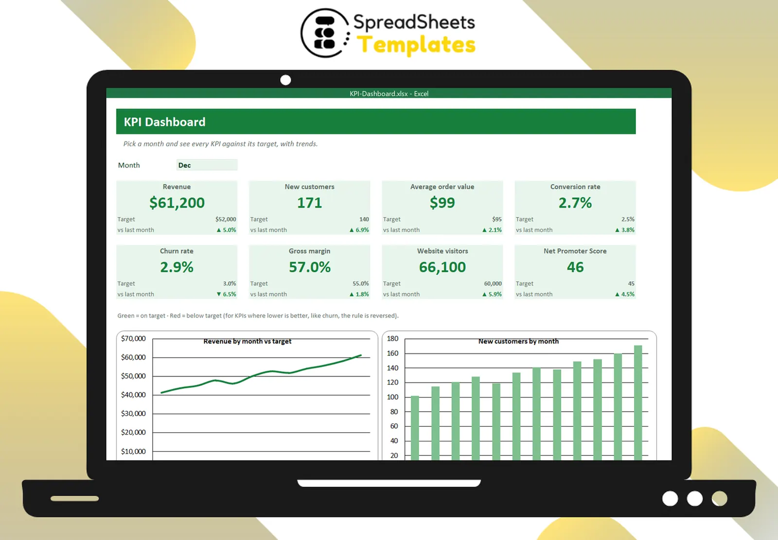
Each card shows:
- the KPI name;
- the value for the selected month (big);
- the target;
- the change vs last month (▲/▼).
Conditional formatting colors the value green when it meets the target and red when it doesn’t — reversed for “lower is better” KPIs.
Step 5: Add one or two trend charts
A line chart of revenue and a bar chart of new customers across the year give context to the cards. Avoid chart overload.
Keep it useful
- Update on the same day every month.
- Review it in a fixed meeting.
- Remove KPIs nobody acts on.
- Write one sentence of commentary per red card.
Template
The KPI Dashboard has a data sheet for 8 KPIs with targets and direction, a month selector, KPI cards with change vs last month and green/red status, and two trend charts.